In this article, some extra mathematical details related to the solution of the steady-state reaction-diffusion equation using PETSc are discussed. First, the simple nonlinear governing equation of interest is shown. Then, Newton’s method is presented at the partial differential equation (PDE) level for generality rather than being presented at the algebraic level. Subsequently, the spatial discretization via the finite difference method is shown for completeness. Finally, a commented PETSc implementation of the discretized reaction-diffusion equation is shown to concretely illustrate how the mathematical notation maps to code.

1. The Governing Equation
2. Newton’s Method at the PDE Level
3. Discretization by the Finite Difference Method
   1. The Residual Form of the PDE
   2. The Jacobian from the Gateaux Derivative
4. Commented Implementation in PETSc
   1. Adapted Implementation
   2. Brief Comment on Original Implementation
5. Conclusion
6. References

The Governing Equation

The general form of the one dimensional, time evolving heat equation can be modelled with diffusion (i.e., \(\frac{\partial^2 u}{\partial x^2}\) in 1D or \(\nabla^2 u\) in N-dimensions), reaction \(R(u)\), and source \(f(\cdot)\) processes for temperature (or substances more generally) with concentration \(u(x, t)\) and is given by

In this post, we focus on the time independent (aka steady state) form of equation (1)

We define also \(R(u) = -\rho \sqrt u\) and \(f(x) = 0\) as well as the Dirichlet boundary conditions \(u(0) = \alpha\) and \(u(1) = \beta\) for our domain \(\Omega \in [0, 1] \).

Clearly, the square root function in \(R(u)\) introduces a nonlinear term into equation (2). Since identifying whether an equation has nonlinear terms naturally determines whether we can use a linear or nonlinear solver, it is useful to recall the definition of a linear operator \(L\) which is said to be linear if, for every pair of functions \(f\) and \(g\) and a scalar \(\theta\)

and

In this case, the square root term is obviously nonlinear. Given this nonlinearity, a nonlinear solver must be used to solve equation (2).

Newton’s Method at the PDE Level

We present here Newton’s method for solving nonlinear equations at the PDE level to make it as generally applicable as possible. Newton’s method is often presented at the algebraic level since its presentation is paired with the discretization (e.g., via finite difference methods, finite element methods, etc.) method of the PDEs. Since there are a large number of techniques to discretize PDEs, it is more general to formulate Newton’s method in the context of the strong (“original”) form of the PDEs. You can then select and apply the appropriate steps for your desired discretization (e.g., for the finite element method, this involves deriving a weak formulation and substituting the finite element solution using specified basis functions) followed by an application of your solver to the discretized PDEs.

Now, Newton’s method is for solving general nonlinear equations of the form

Substituting equation (2) into equation (3) and then expanding terms

we now have our governing equation in the desired general form. A cornerstone of computational science is converting problems into forms that we know how to solve effectively. We know and have numerous methods to solve linear systems of equations. Newton’s method iteratively approximates solutions to \(u\) in equation (4) by linearizing (i.e., converting a nonlinear problem to a linear one) around an iterate, solving the new linear system for a step in the direction of the solution, and then adding that step to the current iterate. That step in the direction of the solution is called a “Newton step” or perturbation. Mathematically, this solution process can be written as

The “linearization” is equation (5.1): it is a truncated Taylor series that is a linear function of \(\delta u\) that approximates \(F\) near \(u^k\) at iteration \(k\), therefore we have replaced our nonlinear function with a linear one. We seek the zero of this function, that is \(F(u^k + \delta u) = 0\) and rearrange to get equation (5.2). The term \(F’(u)(\delta u)\) may look a little suspicious, but consider for a moment what \(F\) actually is. If \(F\) were a scalar function, naturally \(F’\) is the ordinary derivative. Similarly, if \(F\) were a vector function, \(F’\) would be the Jacobian written as \(J_F(u^k)\). However, \(F\) is neither a scalar nor a vector function, but rather it is an operator: a map of one function space to another function space. That is, \(F\) maps the function space of \(u\) to another function space. Thus, we must define the derivative of an operator. This is given by the Gateaux derivative

It turns out that by definition, \(F’\) in \(dF(u; \delta u) = F’(u)(\delta u)\) is just the continuous linear operator represented by the Jacobian matrix (see Rall 1971). Thus, to solve nonlinear PDE problems via Newton’s method, we must do one of the following:

(a) Provide the Jacobian explicitly after deriving and discretizing the Gateaux derivative.

(b) Allow a library (or write it yourself if you so desire) to compute the Jacobian by relying on automatic differentiation (e.g., NonlinearSolver.jl: Solvers) and/or sparsity detection (e.g., NonlinearSolve.jl: Declaring a Sparse Jacobian with Automatic Sparsity Detection).

(c) Allow a library to symbolically compute the Jacobian (e.g., Mathematica: Unconstrained Optimization – Methods for Solving Nonlinear Equations, FENICS: Solving the Nonlinear Variational Problem Directly, etc.).

It is worth noting that there are Jacobian-free methods (see Knoll 2004), but these come with their own trade-offs.

To be as explicit as possible, we now compute the Gateaux derivative of \(F\)

Once we have the Gateaux derivative, equation (5.3) is simply an update of the solution space in the direction “pointing” toward the zero of our nonlinear function.

Discretization by the Finite Difference Method

We now have the continuous forms of the reaction-diffusion equation suitable for solution via Newton’s method. To provide implementations, these continuous forms have to be discretized as shown in the next sections. We therefore define a structured, 1D grid with spacing \(h\) between grid points and indices \(i \in [0…5] \) where the full domain is \(x \in [0, 1]\). Recall also that \(u(0) = \alpha\) and \(u(1) = \beta\). Note that the grid spacing can be calculated by \(h = \frac{1}{m_x - 1}\) where \(m_x\) is the number of grid points. Naturally, we subtract 1 as there are \(m_x - 1\) “spacings” between the \(1^{st}\) and \(m_x^{th}\) grid point. The grid is depicted and annotated below for reference.

                  h
               -------
               |     |
               V     V
u: α     ?     ?     ?     ?     β
   ▆-----▆-----▆-----▆-----▆-----▆
x: 0    0.2   0.4   0.6   0.8    1
i: 0     1     2     3     4     5 

The Residual Form of the PDE

Here, we discretize equation (4). The focus of this article is not on the derivation of the finite difference method, so, if you’re unfamiliar with it, a clear explanation and derivation can be found at CFD University’s: The Finite Difference Method. Ignore the bits in that article related to the Navier-Stokes equations, of course. In any case, the discrete form of the second derivative operator using a centered finite difference is given by

where \(u_i\) the solution at grid point \(i\). That’s it!

The Jacobian from the Gateaux Derivative

Since equation (6) defines a linear operator on \(\delta u\), we only care about discretizing the coefficients of \(\delta u\). That is, we want the discrete form of the continuous linear operator

since \(F’(u)\) acts on \(\delta u\) as represented by \(F’(u)(\delta u)\) in equation (5.2). If we apply a centered finite difference scheme to discretize the second derivative operator on \(\delta u\), we have

For the derivative of the reaction function given by \(\frac{dR}{du}\), \(u\) in \(\frac{\rho}{2 \sqrt u}\) corresponds simply to \(u_i^{k}\) since this is the discrete solution at the grid point \(i\) at Newton step \(k\).

If you’re paying attention, you’ll notice that the discrete form of the second derivative operator—a linear operator—in equation (9) acting on \(\delta u\) is the same as the discrete form of the second derivative operator when it acts on \(u\) in equation (7). This may seem like a rather silly or obvious thing to note; however, it’s surprisingly important for the efficient solution of nonlinear equations since the discrete form of the linear operator is completely independent of the values of \(u_i^k\)—which is changing at every iteration as defined by equation (5.3). This means that a performance-conscious programmer can not only initialize the sparsity pattern of the Jacobian but can also cache those values of the discrete linear operator in the Jacobian—meaning you do not have to assign the coefficients of the discrete linear operator to the Jacobian more than once. This doesn’t apply to the PETSc implementation of the present article, but it’s information that’s certainly worth knowing. You can find an example of this sort of caching in a solving the Navier-Stokes equations with Ferrite.jl example if you like.

With the discrete operations described above, we now frame the action of the Jacobian on the perturbation \(\delta u\) in the context of a Newton iteration \(k\). The Jacobian can therefore be written—emphasizing the coefficients of the Jacobian by wrapping them in brackets—in the form

With the components of the Jacobian explicitly specified, we can now propose functions for implementing the solution of the reaction-diffusion equation using PETSc.

Commented Implementation in PETSc

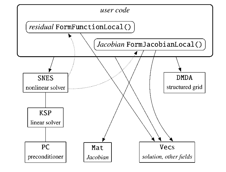
PETSc provides and supports a suite of (non)linear solvers, preconditioners, data types for linear algebra, massive scalability through automatic support for distributed and shared memory parallelism, and much more. The user need only provide a comparatively simple—at least for the problem we consider in this article—set of functions that specify their particular problem. Per figure (1), the user needs to implement FormFunctionLocal—which is simply \(F(u)\)—as well as FormJacobianLocal—which is simply \(J_F(u^k)\). First the implementation will be shown, then relevant parts of the code will be mapped to their mathematical equivalent.

Adapted Implementation

In this section we implement the necessary PETSc functions for the solution of the reaction-diffusion equation. These implementations correspond directly to the maths introduced in the present article.

The PETSc function below for \(F(u)\) is adapted from p4pdes/reaction.c:92-115.

1
2
3
4
5
6
7
8
9
10
11
12
13
14
15
16
17
18
19
20
21
22
23
24
25
26
27
28
29
30
31
32
// Compute F(u) for reaction-diffusion equation
// Reference: Equation (7)
PetscErrorCode FormFunctionLocal(DMDALocalInfo *info, PetscReal *u,
                                 PetscReal *FF, AppCtx *user) {
    PetscInt   i;
    PetscReal  h = 1.0 / (info->mx-1), x, R;
    // iterate through grid indices 
    for (i=info->xs; i<info->xs+info->xm; i++) {
        // point on left boundary
        if (i == 0) {
            FF[i] = u[i] - user->alpha;
        // point on right boundary
        } else if (i == info->mx-1) {
            FF[i] = u[i] - user->beta;
        // interior 
        } else {
            // stencil includes left boundary
            if (i == 1) {
                FF[i] = user->alpha - 2.0 * u[i] + u[i+1]; 
            // stencil includes right boundary
            } else if (i == info->mx-2) {
                FF[i] = u[i-1] - 2.0 * u[i] + user->beta;
            // stencil is purely in interior 
            } else {
                FF[i] = u[i-1] - 2.0 * u[i] + u[i+1];
            }
            R = -user->rho * PetscSqrtReal(u[i]);
            FF[i] = FF[i] / (h*h) + R;
        }
    }
    return 0;
}

In line 6, the grid spacing h is computed as expected. In line 8, we iterate through the locally owned part of a distributed vector, hence the indices start from xs and go until (but excluding) the local index start plus the number of points info->xm owned by the process.

There are, of course, two special cases that occur while iterating over the grid points: the left boundary (i.e., \(u(0) \equiv u_0 = \alpha\)) and the right boundary (i.e., \(u(1) \equiv u_{m_x - 1} = \beta\)) conditions. From equation (4) and equation (7), we know that \(F_i = 0\), and if we recognize the fact that the boundary conditions demand that \(u_0 = \alpha \), then we can infer that \(F_0 = u_0 - \alpha = 0\), which is exactly the residual form we need. Line 11 follows from this reasoning. The same logic applies to line 14 but for the right boundary condition.

Lines 16 to 29 handle the interior points. Line 19 is the discrete second derivative for the second—index i=1—grid point in the 1D grid where on the left boundary \(u_{i-1} = u_{0} = \alpha\). Line 22 is analagous but for the right boundary where \(u_{i+1} = u_{m_x - 1} = \beta \). Line 27 computes the reaction function using its definition. Finally, line 28 divides the numerator of equation (7) that was computed in one of the branches of lines 18 to 26 by the square of the grid size accordingly to complete the computation of the discrete second derivative of \(u\), then the reaction function evaluated in line 27 is added also per equation (7).

Next, the PETSc function for the Jacobian is adapted from p4pdes/reaction.c:117-114.

1
2
3
4
5
6
7
8
9
10
11
12
13
14
15
16
17
18
19
20
21
22
23
24
25
26
27
28
29
30
31
32
33
34
// Compute J_F(u^k) for reaction-diffusion equation
// Reference: Equation (10)
PetscErrorCode FormJacobianLocal(DMDALocalInfo *info, PetscReal *u,
                                 Mat J, Mat P, AppCtx *user) {
    PetscInt   i, col[3];
    PetscReal  h = 1.0 / (info->mx-1), dRdu, v[3];
    for (i=info->xs; i<info->xs+info->xm; i++) {
        // boundary conditions
        if ((i == 0) || (i == info->mx-1)) {
            v[0] = 1.0;
            PetscCall(MatSetValues(P,1,&i,1,&i,v,INSERT_VALUES));
        // interior 
        } else {
            col[0] = i;
            dRdu = -user->rho / (2.0 * PetscSqrtReal(u[i]));
            v[0] = -2.0 / (h*h) + dRdu;

            col[1] = i-1;   
            v[1] = (i > 1) ? 1.0 / (h*h) : 0.0;
        
            col[2] = i+1;   
            v[2] = (i < info->mx-2) ? 1.0 / (h*h) : 0.0;

            PetscCall(MatSetValues(P,1,&i,3,col,v,INSERT_VALUES));
        }
    }
    PetscCall(MatAssemblyBegin(P,MAT_FINAL_ASSEMBLY));
    PetscCall(MatAssemblyEnd(P,MAT_FINAL_ASSEMBLY));
    if (J != P) {
        PetscCall(MatAssemblyBegin(J,MAT_FINAL_ASSEMBLY));
        PetscCall(MatAssemblyEnd(J,MAT_FINAL_ASSEMBLY));
    }
    return 0;
}

Line 6 and 7 are essentially the same as in FormFunctionLocal.

Once again, we handle the boundary conditions in lines 9 to 13. But why assign a value of 1.0 to the first element of a 3-element vector v and then use v to set only a single element of the matrix P?

As in FormFunctionLocal, at the boundaries we have

and

in the discrete form. Though since we’re concerned with using the continuous notation as this is the form you are most likely to encounter, we have of course \(u(0) = \alpha\), which implies that \(F(u(0)) = \alpha \). Given that \(F(u) = 0\) from equation (4), it follows that

In contrast to equation (4), there is obviously no second derivative operator or reaction operator acting on \(u\). What this means is that for \(u(0)\) and \(u(1)\), we can simply compute the derivative with respect to the unknown at the given boundary points such that

and similarly

Returning to the discrete form, if \(F(u) \approx F(u_i) \) from equation (7), it follows that \(F’(u) \approx F’(u_i)\). Therefore, when i = 0, we have \(F’(u_0) = 1\) and when i = mx-1, we also have \(F’(u_{m_x - 1}) = 1\). This means we set only a single element of P corresponding to the indices i, that is P[i][i] = 1.0 since no further elements need to be set to satisfy the discretization of the boundary conditions. Note that &i is used since the MatSetValues expects a pointer. This concludes the discussion of enforcing boundary conditions in the Jacobian.

In lines 13 to 25 we handle the interior points. Lines 14 to 16 define the coefficient of \(\delta u_i\) in equation (10). Note that in the FormJacobianLocal function, u corresponds to the vector of values of the solution u at Newton iteration k. Therefore, u[i] is equivalent to \(u_i^k\). Lines 18 and 19 define the coefficient of \(\delta u_{i-1}\) using equation (10) only if i does not lie on the boundary, that is enforce the PDE on the interior points and eliminate any coupling with boundary points. Lines 21 and 22 are the same principle but for the coefficient \(\delta u_{i+1}\).

Lastly, lines 29 to 32 sets the Jacobian J to P (see SNES: Jacobian Evaluation), meaning J is the matrix from which the preconditioner \(M\) is built. While the Jacobian is usually the same as the matrix from which the preconditioner is built, in principle you could set a different matrix P that may have more desirable properties (e.g., better conditioned) than J. In practice, P is used in conjunction with the specified preconditioner (e.g., Jacobi, ILU, etc.) \(M\) that is used to solve a left (default for Krylov solvers in PETSc) preconditioned system of equations arising from equations (5.2) and (10) such that

To make the preconditioner discussion concrete, if we were to tell PETSc to use a Jacobi preconditioner, then \(M = \text{diag}(J) = \text{diag}(P)\).

With this, we conclude the discussion of the relationship between the mathematics in the first part of the article and the adapted implementation for \(F(u)\) and \(J_F(u^k)\).

Brief Comment on Original Implementation

The adapted implementation in the previous section is based on maths that we derived in the present article with the intention of making the derivation more clear as well as generally applicable to nonlinear PDE problems. However, the basis of the implementation is from Bueler 2021, and for completeness we shortly explain how the original implementation maps to slightly different rearrangements of the maths we covered throughout the rest of the article.

In Bueler 2021, the governing equation is formulated as

and the corresponding implemented discretization by finite differences is

though \(f = 0\) in this problem, so that term may be ignored. In the original code, there is also a flag for including the the derivative of the reaction function in the Jacobian. If the derivative of the reaction function is excluded from the Jacobian, this simplifies the diagonal of the Jacobian, and therefore the resulting matrix \(K \approx J\) is an approximation for the Jacobian with similar spectral characteristics. For simplicity, we omit this flag in the adapted implementation.

Other than these small changes, the adapted implementation differs very little from the original implementation.

Conclusion

In this article, we bridge the gap between continuous nonlinear PDE theory and practical implementation. We cover Newton’s method, Gateaux derivatives, and an application of the finite difference discretization, while providing concrete PETSc code to solve the nonlinear steady-state reaction-diffusion problem. With mathematical and implementation details explicitly treated, hopefully the reader can now more confidently reason about low level numerical codes that they read and write. Future articles will show similar step-by-step mathematical and implementation details for systems of PDEs as well time dependent PDEs.

References

[1] : Bueler, E. Chapter 4: Nonlinear equations by Newton’s Method in PETSc for Partial Differential Equations: Numerical Solutions in C and Python. SIAM 2021.

[2] : Logg, A. et. al. Chapter 1.2: Nonlinear problems in Automated Solution of Differential Equations by the Finite Element Method – The FEniCS Book. Springer 2012

[3] : Heath, M. Chapter 5: Nonlinear equations in Scientific Computing: An Introductory Survey, 2ed. SIAM 2018.

[4] : Bangerth, W. MATH 676 Lecture 31.55 from Colorado State University: Nonlinear problems, part 2 – Newton’s method for PDEs.

[5] : Dokken, J. The FEniCS Tutorial: Custom Newton Solver.